Sfdwhf

The digamma function ψ(z){displaystyle psi (z)},
visualized in discontinuous domain coloring

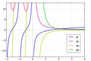
Real part plots of the digamma and the next three polygamma functions along the real line

In mathematics, the digamma function is defined as the logarithmic derivative of the gamma function:^[1][2]

ψ(x)=ddxln⁡(Γ(x))=Γ′(x)Γ(x).{displaystyle psi (x)={frac {d}{dx}}ln {big (}Gamma (x){big )}={frac {Gamma '(x)}{Gamma (x)}}.}

It is the first of the polygamma functions.

The digamma function is often denoted as ψ₀(x), ψ⁽⁰⁾(x) or Ϝ^{[citation needed]} (the uppercase form of the archaic Greek consonant digamma meaning double-gamma).

Relation to harmonic numbers

The gamma function obeys the equation

Γ(z+1)=zΓ(z).{displaystyle Gamma (z+1)=zGamma (z).,}

Taking the derivative with respect to z gives:

Γ′(z+1)=zΓ′(z)+Γ(z){displaystyle Gamma '(z+1)=zGamma '(z)+Gamma (z),}

Dividing by Γ(z + 1) or the equivalent zΓ(z) gives:

Γ′(z+1)Γ(z+1)=Γ′(z)Γ(z)+1z{displaystyle {frac {Gamma '(z+1)}{Gamma (z+1)}}={frac {Gamma '(z)}{Gamma (z)}}+{frac {1}{z}}}

or:

ψ(z+1)=ψ(z)+1z{displaystyle psi (z+1)=psi (z)+{frac {1}{z}}}

Since the harmonic numbers are defined for positive integers n as

Hn=∑k=1n1k,{displaystyle H_{n}=sum _{k=1}^{n}{frac {1}{k}},}

the digamma function is related to them by

ψ(n)=Hn−1−γ,{displaystyle psi (n)=H_{n-1}-gamma ,}

where H₀ = 0, and γ is the Euler–Mascheroni constant. For half-integer arguments the digamma function takes the values

ψ(n+12)=−γ−2ln⁡2+∑k=1n22k−1.{displaystyle psi left(n+{tfrac {1}{2}}right)=-gamma -2ln 2+sum _{k=1}^{n}{frac {2}{2k-1}}.}

Integral representations

If the real part of z is positive then the digamma function has the following integral representation due to Gauss:^[3]

ψ(z)=∫0∞(e−tt−e−zt1−e−t)dt.{displaystyle psi (z)=int _{0}^{infty }left({frac {e^{-t}}{t}}-{frac {e^{-zt}}{1-e^{-t}}}right),dt.}

Combining this expression with an integral identity for the Euler–Mascheroni constant γ{displaystyle gamma } gives:

ψ(z+1)=−γ+∫01(1−tz1−t)dt.{displaystyle psi (z+1)=-gamma +int _{0}^{1}left({frac {1-t^{z}}{1-t}}right),dt.}

The integral is Euler's harmonic number Hz{displaystyle H_{z}}, so the previous formula may also be written

ψ(z+1)=ψ(1)+Hz.{displaystyle psi (z+1)=psi (1)+H_{z}.}

A consequence is the following generalization of the recurrence relation:

ψ(w+1)−ψ(z+1)=Hw−Hz.{displaystyle psi (w+1)-psi (z+1)=H_{w}-H_{z}.}

An integral representation due to Dirichlet is:^[3]

ψ(z)=∫0∞(e−t−1(1+t)z)dtt.{displaystyle psi (z)=int _{0}^{infty }left(e^{-t}-{frac {1}{(1+t)^{z}}}right),{frac {dt}{t}}.}

Gauss's integral representation can be manipulated to give the start of the asymptotic expansion of ψ{displaystyle psi }.^[4]

ψ(z)=log⁡z−12z−∫0∞(12−1t+1et−1)e−tzdt.{displaystyle psi (z)=log z-{frac {1}{2z}}-int _{0}^{infty }left({frac {1}{2}}-{frac {1}{t}}+{frac {1}{e^{t}-1}}right)e^{-tz},dt.}

This formula is also a consequence of Binet's first integral for the gamma function. The integral may be recognized as a Laplace transform.

Binet's second integral for the gamma function gives a different formula for ψ{displaystyle psi } which also gives the first few terms of the asymptotic expansion:^[5]

ψ(z)=log⁡z−12z−2∫0∞tdt(t2+z2)(e2πt−1).{displaystyle psi (z)=log z-{frac {1}{2z}}-2int _{0}^{infty }{frac {t,dt}{(t^{2}+z^{2})(e^{2pi t}-1)}}.}

Infinite product representation

The function ψ(z)/Γ(z){displaystyle psi (z)/Gamma (z)} is an entire function,^[6] and it can be represented by the infinite product

ψ(z)Γ(z)=−e2γz∏k=0∞(1−zxk)ezxk.{displaystyle {frac {psi (z)}{Gamma (z)}}=-e^{2gamma z}prod _{k=0}^{infty }left(1-{frac {z}{x_{k}}}right)e^{frac {z}{x_{k}}}.}

Here xk{displaystyle x_{k}} is the kth zero of ψ{displaystyle psi } (see below), and γ{displaystyle gamma } is the Euler–Mascheroni constant.

Series formula

Euler's product formula for the gamma function, combined with the functional equation and an identity for the Euler–Mascheroni constant, yields the following expression for the digamma function, valid in the complex plane outside the negative integers (Abramowitz and Stegun 6.3.16):^[1]

ψ(z+1)=−γ+∑n=1∞(1n−1n+z),z≠−1,−2,−3,…,=−γ+∑n=1∞(zn(n+z)),z≠−1,−2,−3,….{displaystyle {begin{aligned}psi (z+1)&=-gamma +sum _{n=1}^{infty }left({frac {1}{n}}-{frac {1}{n+z}}right),qquad zneq -1,-2,-3,ldots ,\&=-gamma +sum _{n=1}^{infty }left({frac {z}{n(n+z)}}right),qquad zneq -1,-2,-3,ldots .end{aligned}}}

Equivalently,

ψ(z)=−γ+∑n=0∞(1n+1−1n+z),z≠0,−1,−2,…,=−γ+∑n=0∞z−1(n+1)(n+z),z≠0,−1,−2,…,{displaystyle {begin{aligned}psi (z)&=-gamma +sum _{n=0}^{infty }left({frac {1}{n+1}}-{frac {1}{n+z}}right),qquad zneq 0,-1,-2,ldots ,\&=-gamma +sum _{n=0}^{infty }{frac {z-1}{(n+1)(n+z)}},qquad zneq 0,-1,-2,ldots ,\end{aligned}}}

Evaluation of sums of rational functions

The above identity can be used to evaluate sums of the form

∑n=0∞un=∑n=0∞p(n)q(n),{displaystyle sum _{n=0}^{infty }u_{n}=sum _{n=0}^{infty }{frac {p(n)}{q(n)}},}

where p(n) and q(n) are polynomials of n.

Performing partial fraction on u_n in the complex field, in the case when all roots of q(n) are simple roots,

un=p(n)q(n)=∑k=1makn+bk.{displaystyle u_{n}={frac {p(n)}{q(n)}}=sum _{k=1}^{m}{frac {a_{k}}{n+b_{k}}}.}

For the series to converge,

limn→∞nun=0,{displaystyle lim _{nto infty }nu_{n}=0,}

otherwise the series will be greater than the harmonic series and thus diverge. Hence

∑k=1mak=0,{displaystyle sum _{k=1}^{m}a_{k}=0,}

and

∑n=0∞un=∑n=0∞∑k=1makn+bk=∑n=0∞∑k=1mak(1n+bk−1n+1)=∑k=1m(ak∑n=0∞(1n+bk−1n+1))=−∑k=1mak(ψ(bk)+γ)=−∑k=1makψ(bk).{displaystyle {begin{aligned}sum _{n=0}^{infty }u_{n}&=sum _{n=0}^{infty }sum _{k=1}^{m}{frac {a_{k}}{n+b_{k}}}\&=sum _{n=0}^{infty }sum _{k=1}^{m}a_{k}left({frac {1}{n+b_{k}}}-{frac {1}{n+1}}right)\&=sum _{k=1}^{m}left(a_{k}sum _{n=0}^{infty }left({frac {1}{n+b_{k}}}-{frac {1}{n+1}}right)right)\&=-sum _{k=1}^{m}a_{k}{big (}psi (b_{k})+gamma {big )}\&=-sum _{k=1}^{m}a_{k}psi (b_{k}).end{aligned}}}

With the series expansion of higher rank polygamma function a generalized formula can be given as

∑n=0∞un=∑n=0∞∑k=1mak(n+bk)rk=∑k=1m(−1)rk(rk−1)!akψrk−1(bk),{displaystyle sum _{n=0}^{infty }u_{n}=sum _{n=0}^{infty }sum _{k=1}^{m}{frac {a_{k}}{(n+b_{k})^{r_{k}}}}=sum _{k=1}^{m}{frac {(-1)^{r_{k}}}{(r_{k}-1)!}}a_{k}psi ^{r_{k}-1}(b_{k}),}

provided the series on the left converges.

Taylor series

The digamma has a rational zeta series, given by the Taylor series at z = 1. This is

ψ(z+1)=−γ−∑k=1∞ζ(k+1)(−z)k,{displaystyle psi (z+1)=-gamma -sum _{k=1}^{infty }zeta (k+1)(-z)^{k},}

which converges for |z| < 1. Here, ζ(n) is the Riemann zeta function. This series is easily derived from the corresponding Taylor's series for the Hurwitz zeta function.

Newton series

The Newton series for the digamma, sometimes referred to as Stern series,^[7][8] reads

ψ(s+1)=−γ−∑k=1∞(−1)kk(sk){displaystyle psi (s+1)=-gamma -sum _{k=1}^{infty }{frac {(-1)^{k}}{k}}{binom {s}{k}}}

where (^s
_k) is the binomial coefficient. It may also be generalized to

ψ(s+1)=−γ−1m∑k=1m−1m−ks+k−1m∑k=1∞(−1)kk{(s+mk+1)−(sk+1)},ℜ(s)>−1,{displaystyle psi (s+1)=-gamma -{frac {1}{m}}sum _{k=1}^{m-1}{frac {m-k}{s+k}}-{frac {1}{m}}sum _{k=1}^{infty }{frac {(-1)^{k}}{k}}left{{binom {s+m}{k+1}}-{binom {s}{k+1}}right},qquad Re (s)>-1,}

where m = 2,3,4,...^[8]

Series with Gregory's coefficients, Cauchy numbers and Bernoulli polynomials of the second kind

There exist various series for the digamma containing rational coefficients only for the rational arguments. In particular, the series with Gregory's coefficients G_n is

ψ(v)=ln⁡v−∑n=1∞|Gn|(n−1)!(v)n,ℜ(v)>0,{displaystyle psi (v)=ln v-sum _{n=1}^{infty }{frac {{big |}G_{n}{big |}(n-1)!}{(v)_{n}}},qquad Re (v)>0,}

ψ(v)=2ln⁡Γ(v)−2vln⁡v+2v+2ln⁡v−ln⁡2π−2∑n=1∞|Gn(2)|(v)n(n−1)!,ℜ(v)>0,{displaystyle psi (v)=2ln Gamma (v)-2vln v+2v+2ln v-ln 2pi -2sum _{n=1}^{infty }{frac {{big |}G_{n}(2){big |}}{(v)_{n}}},(n-1)!,qquad Re (v)>0,}

ψ(v)=3ln⁡Γ(v)−6ζ′(−1,v)+3v2ln⁡v−32v2−6vln⁡(v)+3v+3ln⁡v−32ln⁡2π+12−3∑n=1∞|Gn(3)|(v)n(n−1)!,ℜ(v)>0,{displaystyle psi (v)=3ln Gamma (v)-6zeta '(-1,v)+3v^{2}ln {v}-{frac {3}{2}}v^{2}-6vln(v)+3v+3ln {v}-{frac {3}{2}}ln 2pi +{frac {1}{2}}-3sum _{n=1}^{infty }{frac {{big |}G_{n}(3){big |}}{(v)_{n}}},(n-1)!,qquad Re (v)>0,}

where (v)_n is the rising factorial (v)_n =
v(v+1)(v+2) ... (v+n-1), G_n(k) are the Gregory coefficients of higher order with G_n(1) = G_n, Γ is the gamma function and ζ is the Hurwitz zeta function.^[9][8]
Similar series with the Cauchy numbers of the second kind C_n reads^[9][8]

ψ(v)=ln⁡(v−1)+∑n=1∞Cn(n−1)!(v)n,ℜ(v)>1,{displaystyle psi (v)=ln(v-1)+sum _{n=1}^{infty }{frac {C_{n}(n-1)!}{(v)_{n}}},qquad Re (v)>1,}

A series with the Bernoulli polynomials of the second kind has the following form^[8]

ψ(v)=ln⁡(v+a)+∑n=1∞(−1)nψn(a)(n−1)!(v)n,ℜ(v)>−a,{displaystyle psi (v)=ln(v+a)+sum _{n=1}^{infty }{frac {(-1)^{n}psi _{n}(a),(n-1)!}{(v)_{n}}},qquad Re (v)>-a,}

where ψ_n(a) are the Bernoulli polynomials of the second kind defined by the generating
equation

z(1+z)aln⁡(1+z)=∑n=0∞znψn(a),|z|<1,{displaystyle {frac {z(1+z)^{a}}{ln(1+z)}}=sum _{n=0}^{infty }z^{n}psi _{n}(a),,qquad |z|<1,,}

It may be generalized to

ψ(v)=1r∑l=0r−1ln⁡(v+a+l)+1r∑n=1∞(−1)nNn,r(a)(n−1)!(v)n,ℜ(v)>−a,r=1,2,3,…{displaystyle psi (v)={frac {1}{r}}sum _{l=0}^{r-1}ln(v+a+l)+{frac {1}{r}}sum _{n=1}^{infty }{frac {(-1)^{n}N_{n,r}(a)(n-1)!}{(v)_{n}}},qquad Re (v)>-a,quad r=1,2,3,ldots }

where the polynomials N_n,r(a) are given by the following generating equation

(1+z)a+m−(1+z)aln⁡(1+z)=∑n=0∞Nn,m(a)zn,|z|<1,{displaystyle {frac {(1+z)^{a+m}-(1+z)^{a}}{ln(1+z)}}=sum _{n=0}^{infty }N_{n,m}(a)z^{n},qquad |z|<1,}

so that N_n,1(a) = ψ_n(a).^[8] Similar expressions with the logarithm of the gamma function involve these formulas^[8]

ψ(v)=1v+a−12{ln⁡Γ(v+a)+v−12ln⁡2π−12+∑n=1∞(−1)nψn+1(a)(v)n(n−1)!},ℜ(v)>−a,{displaystyle psi (v)={frac {1}{v+a-{tfrac {1}{2}}}}left{ln Gamma (v+a)+v-{frac {1}{2}}ln 2pi -{frac {1}{2}}+sum _{n=1}^{infty }{frac {(-1)^{n}psi _{n+1}(a)}{(v)_{n}}}(n-1)!right},qquad Re (v)>-a,}

and

ψ(v)=112r+v+a−1{ln⁡Γ(v+a)+v−12ln⁡2π−12+1r∑n=0r−2(r−n−1)ln⁡(v+a+n)+1r∑n=1∞(−1)nNn+1,r(a)(v)n(n−1)!},ℜ(v)>−a,r=2,3,4,…{displaystyle psi (v)={frac {1}{{tfrac {1}{2}}r+v+a-1}}left{ln Gamma (v+a)+v-{frac {1}{2}}ln 2pi -{frac {1}{2}}+{frac {1}{r}}sum _{n=0}^{r-2}(r-n-1)ln(v+a+n)+{frac {1}{r}}sum _{n=1}^{infty }{frac {(-1)^{n}N_{n+1,r}(a)}{(v)_{n}}}(n-1)!right},qquad Re (v)>-a,quad r=2,3,4,ldots }

Reflection formula

The digamma function satisfies a reflection formula similar to that of the gamma function:

ψ(1−x)−ψ(x)=πcot⁡πx{displaystyle psi (1-x)-psi (x)=pi cot pi x}

Recurrence formula and characterization

The digamma function satisfies the recurrence relation

ψ(x+1)=ψ(x)+1x.{displaystyle psi (x+1)=psi (x)+{frac {1}{x}}.}

Thus, it can be said to "telescope" 1 / x, for one has

Δ[ψ](x)=1x{displaystyle Delta [psi ](x)={frac {1}{x}}}

where Δ is the forward difference operator. This satisfies the recurrence relation of a partial sum of the harmonic series, thus implying the formula

ψ(n)=Hn−1−γ{displaystyle psi (n)=H_{n-1}-gamma }

where γ is the Euler–Mascheroni constant.

More generally, one has

ψ(1+z)=−γ+∑k=1∞(1k−1z+k).{displaystyle psi (1+z)=-gamma +sum _{k=1}^{infty }left({frac {1}{k}}-{frac {1}{z+k}}right).}

for Re(z)>0{displaystyle Re(z)>0}. Another series expansion is:

ψ(1+z)=ln⁡(z)+12z−∑j=1∞B2j2jz2j{displaystyle psi (1+z)=ln(z)+{frac {1}{2z}}-displaystyle sum _{j=1}^{infty }{frac {B_{2j}}{2jz^{2j}}}},

where B2j{displaystyle B_{2j}} are the Bernoulli numbers. This series diverges for all z and is known as the Stirling series.

Actually, ψ is the only solution of the functional equation

F(x+1)=F(x)+1x{displaystyle F(x+1)=F(x)+{frac {1}{x}}}

that is monotonic on ℝ⁺ and satisfies F(1) = −γ. This fact follows immediately from the uniqueness of the Γ function given its recurrence equation and convexity restriction. This implies the useful difference equation:

ψ(x+N)−ψ(x)=∑k=0N−11x+k{displaystyle psi (x+N)-psi (x)=sum _{k=0}^{N-1}{frac {1}{x+k}}}

Some finite sums involving the digamma function

There are numerous finite summation formulas for the digamma function. Basic summation formulas, such as

∑r=1mψ(rm)=−m(γ+ln⁡m),{displaystyle sum _{r=1}^{m}psi left({frac {r}{m}}right)=-m(gamma +ln m),}

∑r=1mψ(rm)⋅exp⁡2πrkim=mln⁡(1−exp⁡2πkim),k∈Z,m∈N, k≠m.{displaystyle sum _{r=1}^{m}psi left({frac {r}{m}}right)cdot exp {dfrac {2pi rki}{m}}=mln left(1-exp {frac {2pi ki}{m}}right),qquad kin mathbb {Z} ,quad min mathbb {N} , kneq m.}

∑r=1m−1ψ(rm)⋅cos⁡2πrkm=mln⁡(2sin⁡kπm)+γ,k=1,2,…,m−1{displaystyle sum _{r=1}^{m-1}psi left({frac {r}{m}}right)cdot cos {dfrac {2pi rk}{m}}=mln left(2sin {frac {kpi }{m}}right)+gamma ,qquad k=1,2,ldots ,m-1}

∑r=1m−1ψ(rm)⋅sin⁡2πrkm=π2(2k−m),k=1,2,…,m−1{displaystyle sum _{r=1}^{m-1}psi left({frac {r}{m}}right)cdot sin {frac {2pi rk}{m}}={frac {pi }{2}}(2k-m),qquad k=1,2,ldots ,m-1}

are due to Gauss.^[10][11] More complicated formulas, such as

∑r=0m−1ψ(2r+12m)⋅cos⁡(2r+1)kπm=mln⁡(tan⁡πk2m),k=1,2,…,m−1{displaystyle sum _{r=0}^{m-1}psi left({frac {2r+1}{2m}}right)cdot cos {frac {(2r+1)kpi }{m}}=mln left(tan {frac {pi k}{2m}}right),qquad k=1,2,ldots ,m-1}

∑r=0m−1ψ(2r+12m)⋅sin⁡(2r+1)kπm=−πm2,k=1,2,…,m−1{displaystyle sum _{r=0}^{m-1}psi left({frac {2r+1}{2m}}right)cdot sin {dfrac {(2r+1)kpi }{m}}=-{frac {pi m}{2}},qquad k=1,2,ldots ,m-1}

∑r=1m−1ψ(rm)⋅cot⁡πrm=−π(m−1)(m−2)6{displaystyle sum _{r=1}^{m-1}psi left({frac {r}{m}}right)cdot cot {frac {pi r}{m}}=-{frac {pi (m-1)(m-2)}{6}}}

∑r=1m−1ψ(rm)⋅rm=−γ2(m−1)−m2ln⁡m−π2∑r=1m−1rm⋅cot⁡πrm{displaystyle sum _{r=1}^{m-1}psi left({frac {r}{m}}right)cdot {frac {r}{m}}=-{frac {gamma }{2}}(m-1)-{frac {m}{2}}ln m-{frac {pi }{2}}sum _{r=1}^{m-1}{frac {r}{m}}cdot cot {frac {pi r}{m}}}

∑r=1m−1ψ(rm)⋅cos⁡(2ℓ+1)πrm=−πm∑r=1m−1r⋅sin⁡2πrmcos⁡2πrm−cos⁡(2ℓ+1)πm,ℓ∈Z{displaystyle sum _{r=1}^{m-1}psi left({frac {r}{m}}right)cdot cos {dfrac {(2ell +1)pi r}{m}}=-{frac {pi }{m}}sum _{r=1}^{m-1}{frac {rcdot sin {dfrac {2pi r}{m}}}{cos {dfrac {2pi r}{m}}-cos {dfrac {(2ell +1)pi }{m}}}},qquad ell in mathbb {Z} }

∑r=1m−1ψ(rm)⋅sin⁡(2ℓ+1)πrm=−(γ+ln⁡2m)cot⁡(2ℓ+1)π2m+sin⁡(2ℓ+1)πm∑r=1m−1ln⁡sin⁡πrmcos⁡2πrm−cos⁡(2ℓ+1)πm,ℓ∈Z{displaystyle sum _{r=1}^{m-1}psi left({frac {r}{m}}right)cdot sin {dfrac {(2ell +1)pi r}{m}}=-(gamma +ln 2m)cot {frac {(2ell +1)pi }{2m}}+sin {dfrac {(2ell +1)pi }{m}}sum _{r=1}^{m-1}{frac {ln sin {dfrac {pi r}{m}}}{cos {dfrac {2pi r}{m}}-cos {dfrac {(2ell +1)pi }{m}}}},qquad ell in mathbb {Z} }

∑r=1m−1ψ2(rm)=(m−1)γ2+m(2γ+ln⁡4m)ln⁡m−m(m−1)ln2⁡2+π2(m2−3m+2)12+m∑ℓ=1m−1ln2⁡sin⁡πℓm{displaystyle sum _{r=1}^{m-1}psi ^{2}left({frac {r}{m}}right)=(m-1)gamma ^{2}+m(2gamma +ln 4m)ln {m}-m(m-1)ln ^{2}2+{frac {pi ^{2}(m^{2}-3m+2)}{12}}+msum _{ell =1}^{m-1}ln ^{2}sin {frac {pi ell }{m}}}

are due to works of certain modern authors (see e.g. Appendix B in Blagouchine (2014)^[12]).

Gauss's digamma theorem

For positive integers r and m (r < m), the digamma function may be expressed in terms of Euler's constant and a finite number of elementary functions

ψ(rm)=−γ−ln⁡(2m)−π2cot⁡(rπm)+2∑n=1⌊m−12⌋cos⁡(2πnrm)ln⁡sin⁡(πnm){displaystyle psi left({frac {r}{m}}right)=-gamma -ln(2m)-{frac {pi }{2}}cot left({frac {rpi }{m}}right)+2sum _{n=1}^{leftlfloor {frac {m-1}{2}}rightrfloor }cos left({frac {2pi nr}{m}}right)ln sin left({frac {pi n}{m}}right)}

which holds, because of its recurrence equation, for all rational arguments.

Asymptotic expansion

The digamma function has the asymptotic expansion

ψ(z)∼log⁡z−12z+∑n=1∞ζ(1−2n)z2n=log⁡z−12z−∑n=1∞B2n2nz2n,{displaystyle psi (z)sim log z-{frac {1}{2z}}+sum _{n=1}^{infty }{frac {zeta (1-2n)}{z^{2n}}}=log z-{frac {1}{2z}}-sum _{n=1}^{infty }{frac {B_{2n}}{2nz^{2n}}},}

where B_k is the kth Bernoulli number and ζ is the Riemann zeta function. The first few terms of this expansion are:

ψ(z)≈log⁡z−12z−112z2+1120z4−1252z6+1240z8−5660z10+69132760z12−112z14+⋯.{displaystyle psi (z)approx log z-{frac {1}{2z}}-{frac {1}{12z^{2}}}+{frac {1}{120z^{4}}}-{frac {1}{252z^{6}}}+{frac {1}{240z^{8}}}-{frac {5}{660z^{10}}}+{frac {691}{32760z^{12}}}-{frac {1}{12z^{14}}}+cdots .}

Although the infinite sum does not converge for any z, any finite partial sum becomes increasingly accurate as z increases.

The expansion can be found by applying the Euler–Maclaurin formula to the sum^[13]

∑n=1∞(1n−1z+n){displaystyle sum _{n=1}^{infty }left({frac {1}{n}}-{frac {1}{z+n}}right)}

The expansion can also be derived from the integral representation coming from Binet's second integral formula for the gamma function. Expanding t/(t2+z2){displaystyle t/(t^{2}+z^{2})} as a geometric series and substituting an integral representation of the Bernoulli numbers leads to the same asymptotic series as above. Furthermore, expanding only finitely many terms of the series gives a formula with an explicit error term:

ψ(z)=log⁡z−12z−∑n=1NB2n2nz2n+(−1)N+12z2N∫0∞t2N+1dt(t2+z2)(e2πt−1).{displaystyle psi (z)=log z-{frac {1}{2z}}-sum _{n=1}^{N}{frac {B_{2n}}{2nz^{2n}}}+(-1)^{N+1}{frac {2}{z^{2N}}}int _{0}^{infty }{frac {t^{2N+1},dt}{(t^{2}+z^{2})(e^{2pi t}-1)}}.}

Inequalities

When x > 0, the function

log⁡x−12x−ψ(x){displaystyle log x-{frac {1}{2x}}-psi (x)}

is completely monotonic and in particular positive. This is a consequence of Bernstein's theorem on monotone functions applied to the integral representation coming from Binet's first integral for the gamma function. Additionally, by the convexity inequality 1+t≤et{displaystyle 1+tleq e^{t}}, the integrand in this representation is bounded above by e−tz/2{displaystyle e^{-tz}/2}. Consequently

1x−log⁡x+ψ(x){displaystyle {frac {1}{x}}-log x+psi (x)}

is also completely monotonic. It follows that, for all x > 0,

log⁡x−1x≤ψ(x)≤log⁡x−12x.{displaystyle log x-{frac {1}{x}}leq psi (x)leq log x-{frac {1}{2x}}.}

This recovers a theorem of Horst Alzer.^[14] Alzer also proved that, for s ∈ (0, 1),^[15]

1−sx+s<ψ(x+1)−ψ(x+s),{displaystyle {frac {1-s}{x+s}}<psi (x+1)-psi (x+s),}

Related bounds were obtained by Elezovic, Giordano, and Pecaric, who proved that, for x > 0 ,

log⁡(x+12)−1x<ψ(x)<log⁡(x+e−γ)−1x,{displaystyle log(x+{tfrac {1}{2}})-{frac {1}{x}}<psi (x)<log(x+e^{-gamma })-{frac {1}{x}},}

where γ{displaystyle gamma } is the Euler–Mascheroni constant.^[16] The constants appearing in these bounds are the best possible.^[17]

The mean value theorem implies the following analog of Gautschi's inequality: If x > c, where c ≈ 1.461 is the unique positive real root of the digamma function, and if s > 0, then

exp⁡((1−s)ψ′(x+1)ψ(x+1))≤ψ(x+1)ψ(x+s)≤exp⁡((1−s)ψ′(x+s)ψ(x+s)).{displaystyle exp left((1-s){frac {psi '(x+1)}{psi (x+1)}}right)leq {frac {psi (x+1)}{psi (x+s)}}leq exp left((1-s){frac {psi '(x+s)}{psi (x+s)}}right).}

Moreover, equality holds if and only if s = 1.^[18]

Inspired by the harmonic mean value inequality for the classical gamma function, Horzt Alzer and Graham Jameson proved, among other things, a harmonic mean-value inequality for the digamma function:

−γ≤2ψ(x)ψ(1x)ψ(x)+ψ(1x){displaystyle -gamma leq {frac {2psi (x)psi ({frac {1}{x}})}{psi (x)+psi ({frac {1}{x}})}}} for x>0{displaystyle x>0}

Equality holds if and only if x=1{displaystyle x=1}.^[19]

Computation and approximation

The asymptotic expansion gives an easy way to compute ψ(x) when the real part of x is large. To compute ψ(x) for small x, the recurrence relation

ψ(x+1)=1x+ψ(x){displaystyle psi (x+1)={frac {1}{x}}+psi (x)}

can be used to shift the value of x to a higher value. Beal^[20] suggests using the above recurrence to shift x to a value greater than 6 and then applying the above expansion with terms above x¹⁴ cut off, which yields "more than enough precision" (at least 12 digits except near the zeroes).

As x goes to infinity, ψ(x) gets arbitrarily close to both ln(x − 1/2) and ln x. Going down from x + 1 to x, ψ decreases by 1 / x, ln(x − 1/2) decreases by ln (x + 1/2) / (x − 1/2), which is more than 1 / x, and ln x decreases by ln (1 + 1 / x), which is less than 1 / x. From this we see that for any positive x greater than 1/2,

ψ(x)∈(ln⁡(x−12),ln⁡x){displaystyle psi (x)in left(ln left(x-{tfrac {1}{2}}right),ln xright)}

or, for any positive x,

exp⁡ψ(x)∈(x−12,x).{displaystyle exp psi (x)in left(x-{tfrac {1}{2}},xright).}

The exponential exp ψ(x) is approximately x − 1/2 for large x, but gets closer to x at small x, approaching 0 at x = 0.

For x < 1, we can calculate limits based on the fact that between 1 and 2, ψ(x) ∈ [−γ, 1 − γ], so

ψ(x)∈(−1x−γ,1−1x−γ),x∈(0,1){displaystyle psi (x)in left(-{frac {1}{x}}-gamma ,1-{frac {1}{x}}-gamma right),quad xin (0,1)}

or

exp⁡ψ(x)∈(exp⁡(−1x−γ),eexp⁡(−1x−γ)).{displaystyle exp psi (x)in left(exp left(-{frac {1}{x}}-gamma right),eexp left(-{frac {1}{x}}-gamma right)right).}

From the above asymptotic series for ψ, one can derive an asymptotic series for exp(−ψ(x)). The series matches the overall behaviour well, that is, it behaves asymptotically as it should for large arguments, and has a zero of unbounded multiplicity at the origin too.

1exp⁡ψ(x)∼1x+12⋅x2+54⋅3!⋅x3+32⋅4!⋅x4+4748⋅5!⋅x5−516⋅6!⋅x6+⋯{displaystyle {frac {1}{exp psi (x)}}sim {frac {1}{x}}+{frac {1}{2cdot x^{2}}}+{frac {5}{4cdot 3!cdot x^{3}}}+{frac {3}{2cdot 4!cdot x^{4}}}+{frac {47}{48cdot 5!cdot x^{5}}}-{frac {5}{16cdot 6!cdot x^{6}}}+cdots }

This is similar to a Taylor expansion of exp(−ψ(1 / y)) at y = 0, but it does not converge.^[21] (The function is not analytic at infinity.) A similar series exists for exp(ψ(x)) which starts with exp⁡ψ(x)∼x−12.{displaystyle exp psi (x)sim x-{frac {1}{2}}.}

If one calculates the asymptotic series for ψ(x+1/2) it turns out that there are no odd powers of x (there is no x⁻¹ term). This leads to the following asymptotic expansion, which saves computing terms of even order.

exp⁡ψ(x+12)∼x+14!⋅x−378⋅6!⋅x3+1031372⋅8!⋅x5−5509121384⋅10!⋅x7+⋯{displaystyle exp psi left(x+{tfrac {1}{2}}right)sim x+{frac {1}{4!cdot x}}-{frac {37}{8cdot 6!cdot x^{3}}}+{frac {10313}{72cdot 8!cdot x^{5}}}-{frac {5509121}{384cdot 10!cdot x^{7}}}+cdots }

Special values

The digamma function has values in closed form for rational numbers, as a result of Gauss's digamma theorem. Some are listed below:

ψ(1)=−γψ(12)=−2ln⁡2−γψ(13)=−π23−3ln⁡32−γψ(14)=−π2−3ln⁡2−γψ(16)=−π32−2ln⁡2−3ln⁡32−γψ(18)=−π2−4ln⁡2−π+ln⁡(2+2)−ln⁡(2−2)2−γ.{displaystyle {begin{aligned}psi (1)&=-gamma \psi left({tfrac {1}{2}}right)&=-2ln {2}-gamma \psi left({tfrac {1}{3}}right)&=-{frac {pi }{2{sqrt {3}}}}-{frac {3ln {3}}{2}}-gamma \psi left({tfrac {1}{4}}right)&=-{frac {pi }{2}}-3ln {2}-gamma \psi left({tfrac {1}{6}}right)&=-{frac {pi {sqrt {3}}}{2}}-2ln {2}-{frac {3ln {3}}{2}}-gamma \psi left({tfrac {1}{8}}right)&=-{frac {pi }{2}}-4ln {2}-{frac {pi +ln left(2+{sqrt {2}}right)-ln left(2-{sqrt {2}}right)}{sqrt {2}}}-gamma .end{aligned}}}

Moreover, by the series representation, it can easily be deduced that at the imaginary unit,

Re⁡ψ(i)=−γ−∑n=0∞n−1n3+n2+n+1,Im⁡ψ(i)=∑n=0∞1n2+1=12+π2coth⁡π.{displaystyle {begin{aligned}operatorname {Re} psi (i)&=-gamma -sum _{n=0}^{infty }{frac {n-1}{n^{3}+n^{2}+n+1}},\[8px]operatorname {Im} psi (i)&=sum _{n=0}^{infty }{frac {1}{n^{2}+1}}\&={frac {1}{2}}+{frac {pi }{2}}coth pi .end{aligned}}}

Roots of the digamma function

The roots of the digamma function are the saddle points of the complex-valued gamma function. Thus they lie all on the real axis. The only one on the positive real axis is the unique minimum of the real-valued gamma function on ℝ⁺ at x₀ = 7000146163214496800♠1.461632144968.... All others occur single between the poles on the negative axis:

x1=−0.504083008…,x2=−1.573498473…,x3=−2.610720868…,x4=−3.635293366…,⋮{displaystyle {begin{aligned}x_{1}&=-0.504,083,008ldots ,\x_{2}&=-1.573,498,473ldots ,\x_{3}&=-2.610,720,868ldots ,\x_{4}&=-3.635,293,366ldots ,\&qquad vdots end{aligned}}}

Already in 1881, Charles Hermite observed^[22] that

xn=−n+1ln⁡n+O(1(ln⁡n)2){displaystyle x_{n}=-n+{frac {1}{ln n}}+Oleft({frac {1}{(ln n)^{2}}}right)}

holds asymptotically. A better approximation of the location of the roots is given by

xn≈−n+1πarctan⁡(πln⁡n)n≥2{displaystyle x_{n}approx -n+{frac {1}{pi }}arctan left({frac {pi }{ln n}}right)qquad ngeq 2}

and using a further term it becomes still better

xn≈−n+1πarctan⁡(πln⁡n+18n)n≥1{displaystyle x_{n}approx -n+{frac {1}{pi }}arctan left({frac {pi }{ln n+{frac {1}{8n}}}}right)qquad ngeq 1}

which both spring off the reflection formula via

0=ψ(1−xn)=ψ(xn)+πtan⁡πxn{displaystyle 0=psi (1-x_{n})=psi (x_{n})+{frac {pi }{tan pi x_{n}}}}

and substituting ψ(x_n) by its not convergent asymptotic expansion. The correct second term of this expansion is 1 / 2n, where the given one works good to approximate roots with small n.

Another improvement of Hermite's formula can be given:^[6]

xn=−n+1log⁡n−12n(log⁡n)2+O(1n2(log⁡n)2).{displaystyle x_{n}=-n+{frac {1}{log n}}-{frac {1}{2n(log n)^{2}}}+Oleft({frac {1}{n^{2}(log n)^{2}}}right).}

Regarding the zeros, the following infinite sum identities were recently proved by István Mező and Michael Hoffman^[6]

∑n=0∞1xn2=γ2+π22,∑n=0∞1xn3=−4ζ(3)−γ3−γπ22,∑n=0∞1xn4=γ4+π49+23γ2π2+4γζ(3).{displaystyle {begin{aligned}sum _{n=0}^{infty }{frac {1}{x_{n}^{2}}}&=gamma ^{2}+{frac {pi ^{2}}{2}},\sum _{n=0}^{infty }{frac {1}{x_{n}^{3}}}&=-4zeta (3)-gamma ^{3}-{frac {gamma pi ^{2}}{2}},\sum _{n=0}^{infty }{frac {1}{x_{n}^{4}}}&=gamma ^{4}+{frac {pi ^{4}}{9}}+{frac {2}{3}}gamma ^{2}pi ^{2}+4gamma zeta (3).end{aligned}}}

In general, the function

Z(k)=∑n=0∞1xnk{displaystyle Z(k)=sum _{n=0}^{infty }{frac {1}{x_{n}^{k}}}}

can be determined and it is studied in detail by the cited authors.

The following results^[6]

∑n=0∞1xn2+xn=−2,∑n=0∞1xn2−xn=γ+π26γ{displaystyle {begin{aligned}sum _{n=0}^{infty }{frac {1}{x_{n}^{2}+x_{n}}}&=-2,\sum _{n=0}^{infty }{frac {1}{x_{n}^{2}-x_{n}}}&=gamma +{frac {pi ^{2}}{6gamma }}end{aligned}}}

also hold true.

Here γ is the Euler–Mascheroni constant.

Regularization

The digamma function appears in the regularization of divergent integrals

∫0∞dxx+a,{displaystyle int _{0}^{infty }{frac {dx}{x+a}},}

this integral can be approximated by a divergent general Harmonic series, but the following value can be attached to the series

∑n=0∞1n+a=−ψ(a).{displaystyle sum _{n=0}^{infty }{frac {1}{n+a}}=-psi (a).}

See also

• Polygamma function


• Trigamma function


• 
  Chebyshev expansions of the digamma function in Wimp, Jet (1961). "Polynomial approximations to integral transforms". Math. Comp. 15 (74): 174–178. doi:10.1090/S0025-5718-61-99221-3..mw-parser-output cite.citation{font-style:inherit}.mw-parser-output .citation q{quotes:"""""""'""'"}.mw-parser-output .citation .cs1-lock-free a{background:url("//upload.wikimedia.org/wikipedia/commons/thumb/6/65/Lock-green.svg/9px-Lock-green.svg.png")no-repeat;background-position:right .1em center}.mw-parser-output .citation .cs1-lock-limited a,.mw-parser-output .citation .cs1-lock-registration a{background:url("//upload.wikimedia.org/wikipedia/commons/thumb/d/d6/Lock-gray-alt-2.svg/9px-Lock-gray-alt-2.svg.png")no-repeat;background-position:right .1em center}.mw-parser-output .citation .cs1-lock-subscription a{background:url("//upload.wikimedia.org/wikipedia/commons/thumb/a/aa/Lock-red-alt-2.svg/9px-Lock-red-alt-2.svg.png")no-repeat;background-position:right .1em center}.mw-parser-output .cs1-subscription,.mw-parser-output .cs1-registration{color:#555}.mw-parser-output .cs1-subscription span,.mw-parser-output .cs1-registration span{border-bottom:1px dotted;cursor:help}.mw-parser-output .cs1-ws-icon a{background:url("//upload.wikimedia.org/wikipedia/commons/thumb/4/4c/Wikisource-logo.svg/12px-Wikisource-logo.svg.png")no-repeat;background-position:right .1em center}.mw-parser-output code.cs1-code{color:inherit;background:inherit;border:inherit;padding:inherit}.mw-parser-output .cs1-hidden-error{display:none;font-size:100%}.mw-parser-output .cs1-visible-error{font-size:100%}.mw-parser-output .cs1-maint{display:none;color:#33aa33;margin-left:0.3em}.mw-parser-output .cs1-subscription,.mw-parser-output .cs1-registration,.mw-parser-output .cs1-format{font-size:95%}.mw-parser-output .cs1-kern-left,.mw-parser-output .cs1-kern-wl-left{padding-left:0.2em}.mw-parser-output .cs1-kern-right,.mw-parser-output .cs1-kern-wl-right{padding-right:0.2em}
  

References

Constructs such as ibid., loc. cit. and idem are discouraged by Wikipedia's style guide for footnotes, as they are easily broken. Please improve this article by replacing them with named references (quick guide), or an abbreviated title. (January 2019) (Learn how and when to remove this template message)

External links

• 
  OEIS sequence A020759 (Decimal expansion of (-1)*Gamma'(1/2)/Gamma(1/2) where Gamma(x) denotes the Gamma function)—psi(1/2)

OEIS: A047787 psi(1/3), OEIS: A200064 psi(2/3), OEIS: A020777 psi(1/4), OEIS: A200134 psi(3/4), OEIS: A200135 to OEIS: A200138 psi(1/5) to psi(4/5).